Introduction
In this post I´ll explore some basic approaches to analyze a simple simulated data example.
Two sample continuous outcome
Consider a dependent variable Y and an independent variable X (two levels, A and B). Standardize Y to get zero mean and unit standard deviation.
DAT <- tibble(N = 60 ,
              X = rbinom(N, 1, 0.5),
              Y =  0.5*X + rnorm(N)) %>%
        mutate(X = factor(X, labels = c("A", "B")) ,
               Y = (Y-mean(Y, na.rm=T))/sd(Y, na.rm=T))
Describe the data (recall that Y has been standardized)
DESC <- DAT %>%   group_by(X) %>%
  summarise( mean = mean(Y, na.rm=T) ,
             sd = sd(Y, na.rm=T) ,
             min=min(Y, na.rm=T),
             max=max(Y, na.rm=T) ,
             n = n()) %>%
  knitr::kable(digits = 2)
DESC| X | mean | sd | min | max | n |
|---|---|---|---|---|---|
| A | -0.37 | 0.93 | -2.35 | 1.36 | 19 |
| B | 0.17 | 0.99 | -1.22 | 2.67 | 41 |
Plot the data
PLT_1 <- DAT %>%          ggplot(  aes(x=Y, color=X , fill=X )) +
  #   geom_histogram(aes(y=..density..), position="identity", alpha=0.2 , binwidth= 0.333)+
  geom_density(alpha=0.2)+
  scale_color_manual(values=c("red", "blue"))+
  scale_fill_manual(values=c("red", "blue"))+
  labs(x="Y", y = "Density")+
  theme_classic() +
  geom_rug() +
  theme(legend.text = element_text(size = 12, colour = "black", angle = 0)) +
  theme(legend.position = c(0.8, 0.8)) +
  theme(axis.text.x = element_text(size=12), axis.text.y = element_text(size=12))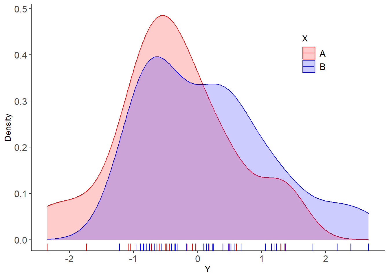
Frequentist inference by a standard linear model (two-sample t-test):
m1 <- broom::tidy(lm(Y~X , data = DAT), conf.int = T,  conf.level = 0.95)[2,]
M <- signif(as.numeric(m1[, 2]) , digits = 2) ;
L<- signif(as.numeric(m1[, 6]) , digits = 2) ;
U <- signif(as.numeric(m1[, 7]), digits = 2) ;
UU_ <- paste( U,"(95%CI:",L, ";",U, ")")
Mean difference and 95% compatibility intervals:
[1] "1.1 (95%CI: 0.0036 ; 1.1 )"Bayesian inference:
Let us use the brms package. Use default priors (what is a default prior?)
library(brms)m13 <- brms::brm(Y ~ X, data = DAT,
family = gaussian,
iter = 4000, warmup = 1000, chains = 4, seed = 12 , cores = 1)Look what was the default priors:
prior_summary(m13)## prior class coef group resp dpar nlpar bound
## (flat) b
## (flat) b XB
## student_t(3, -0.2, 2.5) Intercept
## student_t(3, 0, 2.5) sigma
## source
## default
## (vectorized)
## default
## defaultTry another types of priors:
get_prior(Y ~ X, data = DAT)

priors2 <- c(set_prior("normal(0, 1)", class = "Intercept"),
             set_prior("normal(0, 1)", class = "b", coef = "XB"),
             set_prior("exponential(1)", class = "sigma"))

m14 <- brm(formula = Y ~ X,
             data    = DAT,
             seed    = 123,
              prior = priors2)
Did they model actually use the priors I specified?
prior_summary(m14)## prior class coef group resp dpar nlpar bound source
## (flat) b default
## normal(0, 1) b XB user
## normal(0, 1) Intercept user
## exponential(1) sigma userresA <- fixef(m13)
resB <- fixef(m14)[2,]
M2 <- signif(as.numeric(fixef(m14)[2, 1]) , digits = 2) ;
L2<- signif(as.numeric(fixef(m14)[2, 3]) , digits = 2) ;
U2 <- signif(as.numeric(fixef(m14)[2, 4]), digits = 2) ;
U_2 <- paste( M2,"(95%CI:",L2, ";",U2, ")")So using the same priors, we now get:
U_2## [1] "0.51 (95%CI: 0.0037 ; 1 )"Lets say I have a strong prior belief that the mean difference between A and B is close to one. Let the prior reflect this belief and then estimate the model.
priors3 <- c(set_prior("normal(0, 1)", class = "Intercept"),
             set_prior("normal(1, 0.25)", class = "b", coef = "XB"),
             set_prior("exponential(1)", class = "sigma"))
m15 <- brm(formula = Y ~ X,
             data    = DAT,
             seed    = 123,
              prior = priors3)
Plotting the posterior distribution using the tidybayes package
PPP <- posterior_samples(m15) %>%
  ggplot(aes(x = b_XB , y = 0)) +
  stat_halfeye(fill = "orange2", .width = .95) +
  scale_y_continuous(NULL, breaks = NULL) +
  theme_fivethirtyeight() +
  theme(axis.text.x = element_text( size = 15))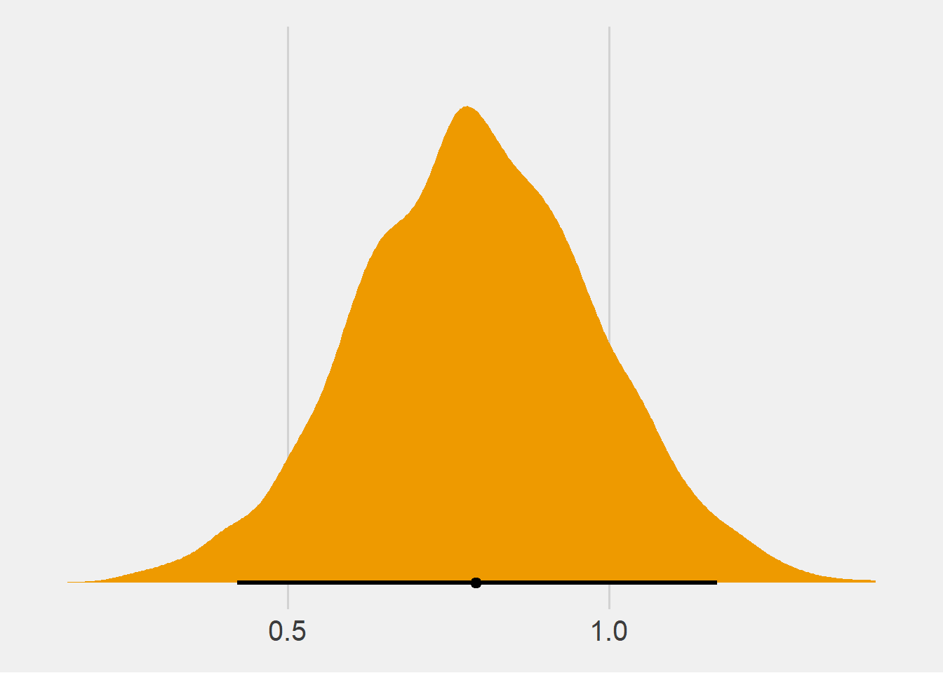
Extract the posterior distributions from the three models (default priors, mean zero prior and mean one prior). I took the code below from here.
set.seed(535)
posterior1.2.3 <- bind_rows("Default priors" = as_tibble(posterior_samples(m13)$b_XB ),
"Mean Zero prior" = as_tibble(posterior_samples(m14)$b_XB ),
"Mean one prior" = as_tibble(posterior_samples(m15)$b_XB ),
.id = "id1") %>%
rename(b_XB = value)
prior1.2.3 <- bind_rows("Default priors" = enframe(runif(10000, min = -2.1, max = 2.1)),
"Mean Zero prior" = enframe(rnorm(10000, mean=0, sd=1)),
"Mean one prior" = enframe(rnorm(10000, mean=1, sd=0.25)),
.id = "id1") %>%
rename(b_XB = value)
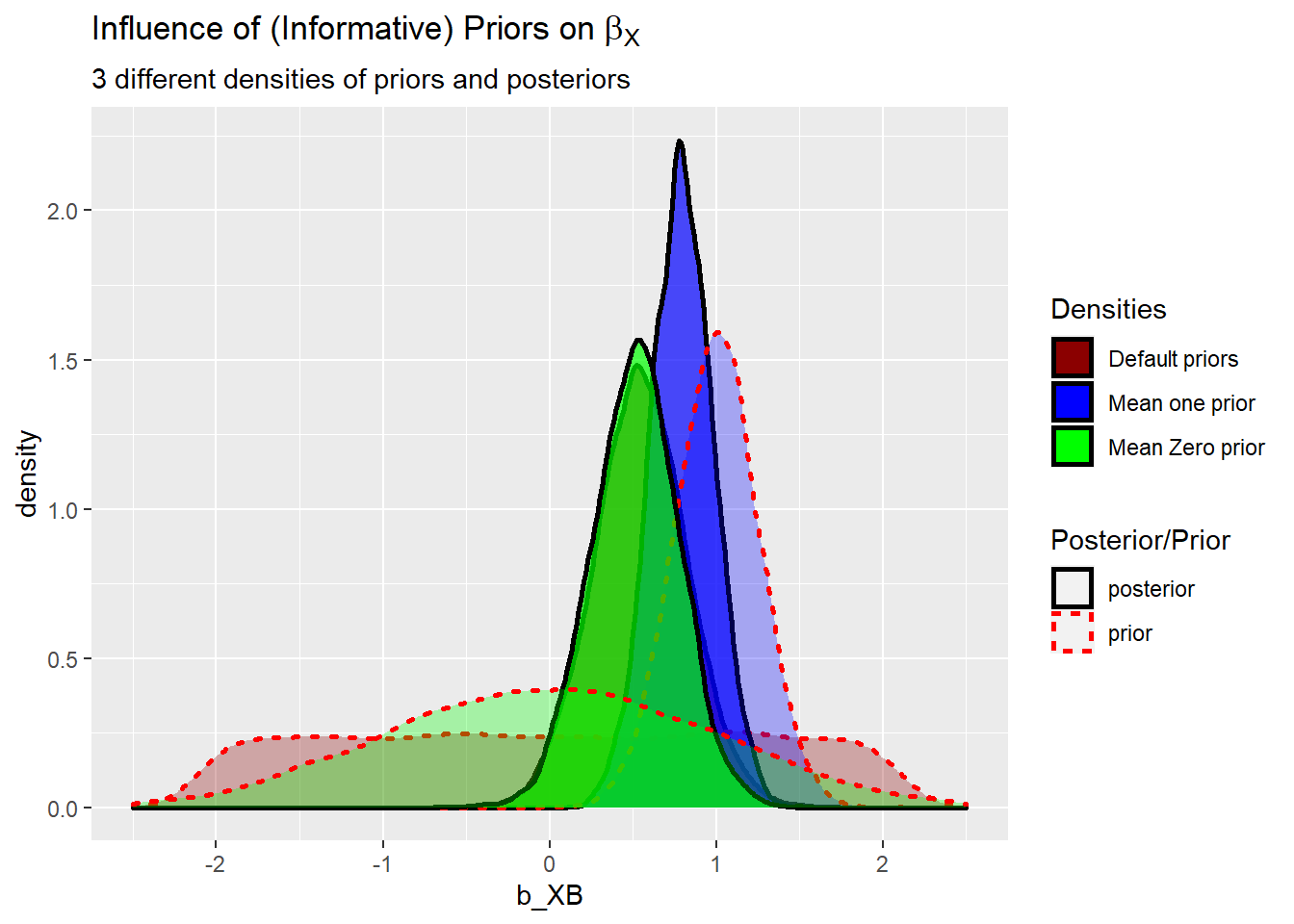
priors.posterior <- bind_rows("posterior" = posterior1.2.3, "prior" = prior1.2.3, .id = "id2")Plot the data. Dotted lines are priors and solid lines are posterior. Default flat (“improper”, that is a prior that is does not fulfill the requirements of a probability distribution) prior and Mean zero prior give very similar posterior. For the mean one prior you see that the posterior is in between the mean of one and the frequentist estimate of 0.53.
PLT_3 <- ggplot(data    = priors.posterior,
       mapping = aes(x        = b_XB,
                     fill     = id1,
                     colour   = id2,
                     linetype = id2,
                     alpha    = id2)) +
  geom_density(size=1)  +
  scale_x_continuous(limits=c(-2.5, 2.5)) +
  scale_colour_manual(name   = 'Posterior/Prior',
                      values = c("black","red"),
                      labels = c("posterior", "prior")) +
  scale_linetype_manual(name   = 'Posterior/Prior',
                        values = c("solid","dotted"),
                        labels = c("posterior", "prior")) +
  scale_alpha_discrete(name   ='Posterior/Prior',
                       range  = c(.7,.3),
                       labels = c("posterior", "prior")) +
  scale_fill_manual(name   = "Densities",
                    values = c("darkred","blue", "green" )) +
  labs(title    = expression("Influence of (Informative) Priors on" ~ beta[X]),
       subtitle = "3 different densities of priors and posteriors")

PLT_3