Frequentist sample size calculation

In order to make an an assertion that \(\theta\)\(>0 (\)\(H_{1})\), if \(\alpha\) =2.5%, \(\sigma\)=2 and we require 80% power to declare statistical significance (make an “assertion of efficacy”, to quote Frank Harrell, watch it here) if the true value of \(\theta\) = 1, then 63 evaluable subjects/group are needed. The (frequentist) probability conditional on \(\theta\) = 1 of rejecting \(H_{0}\), \(P(\text{reject } H_{0}| \theta=1)\) is then 0.80. To achieve \(P(\text{reject } H_{0}| \theta=1)\)=0.90, 84 subjects/group are needed.

Semi-bayesian probability of success (“assertion of efficacy”/Assurance)

Lets say (Gelman, et al)

\[\begin{align*} \theta|\sigma^2 &\sim {\sf N}(\theta_{0}, \tau^2_{0}) \end{align*}\]

\[\begin{align*} \sigma^2 &\sim {\sf Inv-\chi^2}(\nu_{0}, \sigma^2_{0}) \end{align*}\]

The hyperparameters \(\theta_{0}\), \(\tau_{0}\), \(\nu_{0}\), \(\sigma_{0}\) are determined by information from a previous study. Let say the previous study had n=50/group, \(\overline{x}_{1} - \overline{x}_{2}\) = 0.5 and \(\hat{\sigma}\) = 2 for both groups. Then we can calculate the unconditional probability of rejecting \(H_{0}\).

\[\begin{align*} P(\text{reject }H_{0})= \int_{\theta, \sigma}{P(\text{reject }H_{0}| \theta, \sigma^2)\cdot P(\theta, \sigma^2)d\theta\sigma} \end{align*}\]

This is the approach referred to as Assurance proposed by Spiegelhalter & Freedman and developed by O´Hagan. The R package here was used for calculations:

library(assurance)
initial.data <- new.gaussian(delta.mu=0.5, sd1=2, sd2=2, m1=50, m2=50)
later.study <- new.twoArm(size=study.size(grp1.size=63, grp2.size=63),significance=0.05)
Assurance <- round(100*assurance(initial.data, later.study, 100000))

Given the results from the previous study, \(P(\text{reject }H_{0})\)=35%. Given everything else equal, if the previous study had an observed effect of 1 instead of 0.5, then \(P(\text{reject }H_{0})\)=70%. How does the probability of success depend on the sample sizes from the previous and forthcoming study? How does the previously estimated effect influence? Given \(\hat{\sigma}\) = 2, we see that the larger the sample size of the previous study, the less will the assurance be in the in-between uncertain region around 50%. If the previously estimated effect is small (left panel) the assurance will decrease with study size.

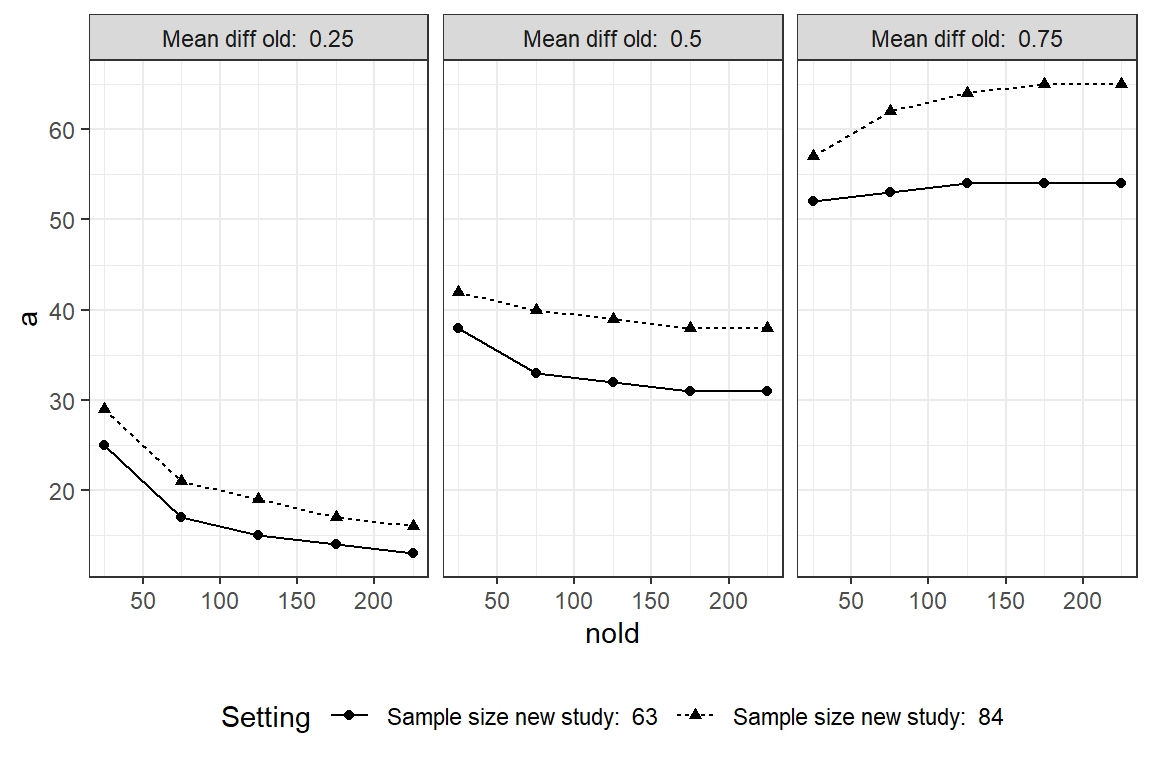
Assurance will increase if the previous estimate indicate a larger effect. For a future study with 63 subjects/group a previous estimated effect of 1 based on a enormous study (>1000 subjects) the assurance will be 80% (the power). With 84 subjects assurance will be 90%. With a previous estimate of 0 assurance will tend to 2.5%.

Hmisc function gbayes2

gbayes2 also refer to Spiegelhalter and Freedman (1986) to compute the probability of correctly concluding that a new treatment is superior to a control. In the Hmisc manual it says “Even though gbayes2 assumes that the test statistic has a normal distribution with known variance (which is strongly a function of the sample size in the two treatment groups), the prior distribution function can be completely general.”. I interpret that the scale parameter \(\sigma\) of the likelihood has a prior with a spike at the value of anticipated standard error of the planned study, i.e. a constant. But this is in practice no limitation because the scale is a nuisance parameter and prior information of \(\theta\) is only what interests us. I think the reason why we can still get closed form solutions without a conjugate prior distribution (we don´t estimate a posterior distribution here, though) is because is fixed \(\sigma\) (for the same reason Assurance relies on simulations) Assurance, is in principle gbayes2 but where the source of the prior belief (the previous study) is explicitly included, but this is of course not needed.

Again, given the previous study with n=50/group, \(\overline{x}_{1} - \overline{x}_{2}\) = 0.5 and \(\hat{\sigma}\) = 2. If we let

\[\begin{align*} \tau|n, \sigma = \sqrt{\frac{2\sigma^2}{n}}= \sqrt{\frac{2\cdot 2^2}{50}}=0.40 \end{align*}\]

library(Hmisc)
N<- 63
SD <- 2
SE <- sqrt(2/N)*SD;

prior0 <- function(delta)dnorm(delta, 0.5, sqrt(2/50)*2)
gb0<-round(100*gbayes2(sd = SE, prior = prior0, delta.w=0, alpha=0.05, upper=Inf))

prior1 <- function(delta)dnorm(delta, 1, sqrt(2/50)*2)
gb1<-round(100*gbayes2(sd = SE, prior = prior1, delta.w=0, alpha=0.05, upper=Inf)) 

prior1 <- function(delta)dnorm(delta, 1, 0.005)
gb2<-round(100*gbayes2(sd = SE, prior = prior1, delta.w=0, alpha=0.05, upper=Inf)) 

Then the probability to achieve a statically significant result in the planned study is 35. If the previous estimated effect was instead 1 then we get 71%. Hence, we get the same results as in the calculates above. Similarly, if the previous study was gigantic, the prior uncertainty is minimal and the probability of success will be equal to the power of the study. Previous setting have had a rather informative prior reflected belief with high certainty as reflected by a small value of the hyperparameter \(\tau\)=0.40. We can allow for more uncertainty by using a vague prior with large value of \(\tau\), say 10.

N<- 63
SD <- 2
SE <- sqrt(2/N)*SD;
prior0 <- function(delta)dnorm(delta, 0.5, 10)
gb3<-round(100*gbayes2(sd = SE, prior = prior0, delta.w=0, alpha=0.05, upper=Inf))

Then we get 49% which is higher than 35% because we now get more of the distribution in the right tail that favor a rejection of \(H_{0}\).

Simulating future studies based on prior predictive distribution

The calculations above combines Bayesian and frequentist philosophies. Since no data is being used (the previous study is just a metaphor for prior belief, it doesn´t matter how we got the information) and no posterior distribution is calculated. An alternative way is to make predictions from the prior distribution and evaluate the operating characteristics of these. This is called the prior predictive distribution.

\[\begin{align*} f(Y)= \int_{\theta, \sigma}{f(Y| \theta, \sigma^2)\cdot P(\theta, \sigma^2)d\theta\sigma} \end{align*}\]

Lets say

\[\begin{align*} Y &\sim {\sf N}(\theta_{0}, \tau^2_{0}) \end{align*}\] \[\begin{align*} \theta_{0} &\sim {\sf N}([0, 0.5], 1) \end{align*}\] \[\begin{align*} \tau_{0} &\sim {\sf half-t}(3, 0.5, 2.5) \end{align*}\]

The prior mean value of \(\theta_{0}\) is hence 0 and 0.5 for group A and B, respectively. We also evaluate for the prior \(\theta_{0}\sim{\sf N}([0, 1.0], 1)\) that is a mean difference of 1.0. The prior for \(\sigma\) is the default prior in the BRMS package.

By combining these prior distributions we can simulate data that is predictions of observations in future studies.

gc()
library(brms)
library(tidybayes)
library(tidymodels)

# Create dummy data for use when making the predictions from the prior
Empty <- tibble(Y = c(0, 0) , X = factor(c(0, 1), labels = c("A", "B")))

# Two scenarios: prior mu = 0.5 and 0.75.
prior_1 = c( prior(normal(0, 1), class = "b", coef = "XA"),
             prior(normal(0.5, 1), class = "b", coef = "XB") )  
prior_2 = c( prior(normal(0, 1), class = "b", coef = "XA"),
             prior(normal(1, 1), class = "b", coef = "XB") )  

fnc <- function(sz, P_, MU)
{
# Specify priors
prior_ = P_     
# Set up the model to simulate from
BPr <-   brms::brm(data = Empty,
                   family = gaussian,
                   Y ~  0 + X,
                   prior = prior_,
                   sample_prior = TRUE ,
                   iter = 4000, warmup = 1000, chains = 4, cores = 4,
                   seed = 12)
# Make predictions of outcomes in future study based on the prior distribution
draws_prior <- Empty %>%
  tidybayes::add_fitted_draws(BPr, n = 10000) %>%
  mutate( Y  = .value) %>%
  dplyr::select(Y, X, .draw, .row) 

df <- data.frame(draws_prior)
# Make repeated (1000 times) samples (i.e. "future studies") of given size. 
  df <- data.frame(draws_prior)
  dfA <- subset(df, X=="A")
  dfB <- subset(df, X=="B")
  smplA <-  infer::rep_sample_n( dfA, size=sz, replace = T, reps = 1000, prob = NULL)
  smplB <-  infer::rep_sample_n( dfB, size=sz, replace = T, reps = 1000, prob = NULL)
  smpl0 <- rbind(smplA, smplB)
  
  smpl <- smpl0 %>% 
    group_by(replicate, X) %>%
    summarise(Average=mean(Y), SD=sd(Y), n=n()) %>%
    group_by(replicate) %>%  
    mutate(Previous = lag(Average), 
           Mean_diff = Average - Previous, 
           LCL = Mean_diff - 1.96*sqrt(2/sz)*SD, 
           Reject=if_else(LCL<0, 0, 1)) %>%
  filter(X=="B") %>%
  mutate(Study.size = paste("N/group: ", sz, "Prior effect ", MU))
  
  LST <- c(draws_prior, smpl)
   return(LST)
  
}
# Percent of times lower 95% confidence interval is > 0
PoS1 <- fnc(sz=63, P_ = prior_1, MU=0.5)
  gc()
PoS2 <- fnc(sz=63, P_ = prior_2, MU=1.0)


PoS1A <- tibble(Y=PoS1$Y, X=PoS1$X)
PoS1B <- tibble(Mean_diff=PoS1$Mean_diff, Reject=PoS1$Reject, Study.size=PoS1$Study.size)
PoS2A <- tibble(Y=PoS2$Y, X=PoS2$X)
PoS2B <- tibble(Mean_diff=PoS2$Mean_diff, Reject=PoS2$Reject, Study.size=PoS2$Study.size)


PoS11 <- round(100*(sum(PoS1B$Reject)/1000))
PoS21 <- round(100*(sum(PoS2B$Reject)/1000))
PoS<- rbind(PoS1B, PoS2B)

# Plot prior predictive distribution
fig2 <- ggplot(PoS1A, aes(x=X, y=Y)) + 
   theme_bw() +
  geom_violin() + 
  geom_boxplot(width=0.1) 

# Plot the distribution of the mean differences
fig3 <- ggplot(PoS, aes(x= Mean_diff, color=Study.size)) +
  geom_density(aes(linetype=Study.size, color=Study.size), size=2) + 
  theme_bw() +
  theme(legend.position="bottom")  + 
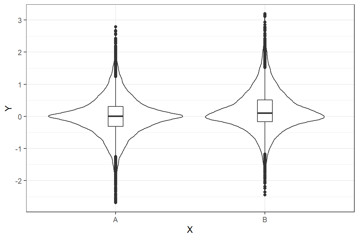
  geom_vline(aes(xintercept=0), color="gray", linetype="dashed", size=1) 

The graph shows the prior predictions for \(\theta_{0}\sim{\sf N}([0, 0.5], 1)\). It is clear that for the current choice of priors data is far from normal - looks more like a double exponential distribution.

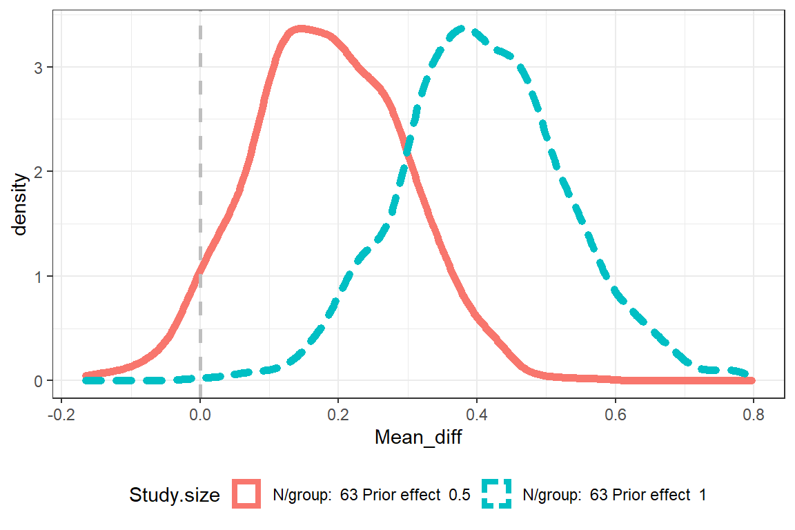
We see that for the prior \(\theta_{0}\sim{\sf N}([0, 0.5], 1)\) and a study size of 63 groups, Assurance (percent of times lower 95% CI is > 0) becomes 37%. For \(\theta_{0}\sim{\sf N}([0, 1.0], 1)\) it becomes 94%.

The plot shows the densities for the mean difference \((\overline{x}_{1} - \overline{x}_{2})\).

The Assurance does not become the same as in the previous calculations. There may be different reasons for this, e.g. how the priors was specified.