Introduction
This is the second of three posts that address:
1. Predicting the probability of a “positive” (reject \(H_{0}\)) study before running the study
2. Interim analyses during the study
3. Evaluating study data in a meaningful way after the study is completed.
The first post is available here.
Interim analyses of an ongoing clinical trial enable early stopping due to efficacy or futility. Clinical trials that involve interims data looks are often referred to as group seque ntial trials. Interim analyses during the course of the study are sound both from an ethical (do not expose subjects to interventions with uncertain risk/benefit more than necessary) and economic (early stopping may reduce costs) point of view. If the repeated interim analyses are made by a frequentist approach, the outcomes from these analyses are difficult to interpret, e.g. regarding observed p-values. When the analyses are performed by a Bayesian approach this difficulty does not arise and the interpretation of the calculated posterior distribution is straightforward. An in-depth discussion on this topic is beyond the scope of this post but will be addressed in a later post.
Prof. Frank Harrell published a post on Statistical Design and Analysis Plan for Sequential Parallel-Group RCT for COVID-19 here where he illustrates by means of simulations how to make interim decisions by continuously updating the posterior distribution of treatment efficacy. To what extent decisions are influenced by different specifications of the prior distributions are demonstrated. The outcome variable is on the ordinal scale. As always, with it comes to Harrell, the work is excellent and very easy to adopt. I have used this work to design a forthcoming RCT of patients with rectal cancer that aims to evaluate different diagnostic tools.
In this post I will use Harrell´s approach to illustrate how to perform interim analyses on an continuous outcome using the same general linear model as in the previous post. I will both use simulated data real data, using the study data from the OPT study.
See also here
Statistical model
Consider the same general linear model as in the previous post:
\[\begin{align*} Y_{i}\sim{\sf N}(\tau_{i}, \sigma_{Y}) \end{align*}\] where \(\sum\tau=0\), j=1, 2. The aim is to estimate \(\theta=\tau_{2}-\tau_{1}\). The estimator \(\overline{x}_{1} - \overline{x}_{2}\) of \(\theta\) is distributed as
\[\begin{align*} {\sf N}(\theta,\sqrt{\frac{2\sigma_{Y}^2}{n}} ) \end{align*}\] where \(n\) is the number of observations for each factor level 1 and 2.
Prior distribution
When specifying a prior distribution for \(\theta\) we adopt Harrell´s approach, i.e.
\[\begin{align*} \theta\sim{\sf N}(0, \sigma_{\theta}) \end{align*}\]
where \(\sigma_{\theta}\) is set such that \({\sf P}(\theta> 1.75) = {\sf P}(\theta< -1.75) = 0.1\). This is relatively informative prior as the distribution is rather compressed. We also consider a less informative one where \({\sf P}(\theta> 1.75) = {\sf P}(\theta< -1.75) = 0.2\) and finally a more or less flat prior, \({\sf P}(\theta> 1.75) = {\sf P}(\theta< -1.75) = 0.45\).
p1<-round(sqrt(((1.75-0)/qnorm(1-0.1))^2), digits=1)
p2<-round(sqrt(((1.75-0)/qnorm(1-0.2))^2), digits=1)
p3<-round(sqrt(((1.75-0)/qnorm(1-0.45))^2), digits=1)
We see that \(\sigma_{\theta}\) = 1.4, 2.1 and 13.9 satisfy these specifications. The parameter \(\sigma_{Y}\) is for our problem a nuisance parameter and is for simplicity assumed fixed, where we plug in the estimated SD obtain from data at the interim looks. At this stage it could be good to simulate observations from the prior distribution to see if they can give rise to data that are at least reasonable. We will however skip this stage.
Go/No Go criteria
At each interim look, declare early stopping due to efficacy if: \[\begin{align*} {\sf P}(\theta>1|data)>0.9 \end{align*}\] Declare early stopping due to futility/harm if \[\begin{align*} {\sf P}(\theta>1|data)<0.2 \end{align*}\] Continue otherwise that is \[\begin{align*} \ 0.2<{\sf P}(\theta>1|data)<0.9 \end{align*}\]
Simulation experiment
Consider a two group parallel group design where 84 subjects/group will yield 90% power to detect a true difference of \(\theta=\tau_{2}-\tau_{1}\) of 1 (given σ=2). Assume the target number of evaluable number of subjects are 90/group and specify a interim analysis scheme that consists of 15 looks with accumulated number of subjects: (6, 12, 18, …, 90 subjects per group, i.e. a total of 12, 24, 36, …, 180). The number of patients used for analysis is hence cumulative, such that all patients (except for the last 12) contribute at least two times. This is all fine since the bayesian approach relies on the likelihood principle.
Performing interim looks with this high intensity is often not be feasible in practice for logistic reasons but is used here for illustration. The code below is taken from Harrell´s post and partly changed to the tidyverse framework.
Note that the simulations below as well as those in Harrell´s post are actually simulations with a single replicate, that is a single dataset is constructed and evaluated for each scenario. A more through evaluation would account for inter-study variability by adding an additional loop around everything. But the current simulations are sufficient for illustration.
Simulate data
# Specifications
LKS <- 15 # Number of looks
N <- 12*LKS # Number of subjects
last_N <- N +1
scenarios=6 # Number of different true effects considered
theta <- c(0, 1/2, 1, 3/2, 2, 5/2) # true mean difference to consider
library(tidyverse)
# Simulate data
set.seed(512)
DATA <- tibble( subj=rep(seq(1:N), times=scenarios),
scenario=sort(rep(theta, times = N)),
X=rep(c(0, 1), times = N*scenarios/2),
my = X*scenario,
Y = rnorm(N*scenarios, mean=my, sd=2),
Group=factor(X, labels=c("Control", "Test")),
lks = rep(sort(rep(seq(1:LKS), times=N/LKS)), times=scenarios),
lksrev = (LKS+1)+desc(lks)) %>%
dplyr::select(subj, scenario, Group, Y, lksrev)
# Group the patients into the different sets being analysed at each interim look.
DATA2 <- DATA %>%
group_by(scenario) %>%
uncount(lksrev) %>%
group_by(scenario, subj) %>%
mutate(lks = (LKS+1)+desc(row_number()))
# Calculate the sufficient statistics at each interim look
DATA3 <- DATA2 %>%
group_by(scenario, Group, lks) %>%
mutate(lks_group=row_number()) %>%
group_by(scenario, lks, Group) %>%
summarise(Mean =mean(Y), sd=sd(Y), n=n()) %>%
mutate(Previous = lag(Mean),
Mean_diff = Mean - Previous,
SE = sqrt(2/n)*sd)
# Difference in means and it´s Standard errors
#(to use in the calculation of the posterior probability)
DATA4 <- DATA3 %>%
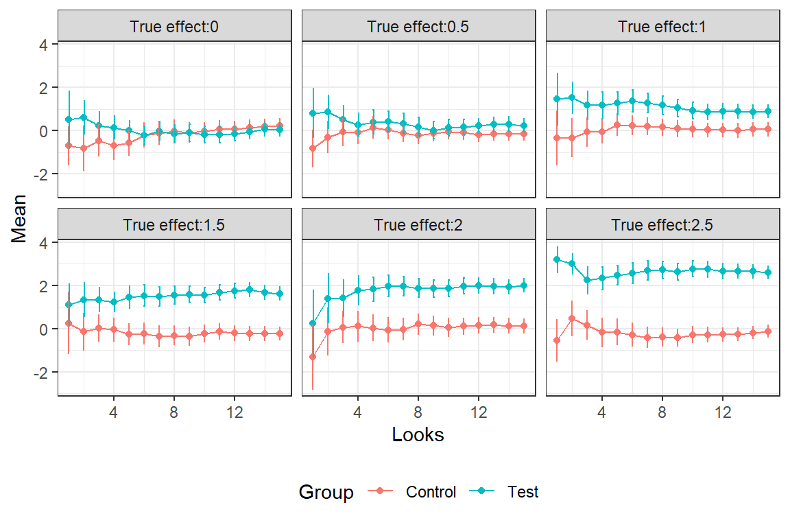
filter(Group == "Test")In the graph we see the estimated averages and 2*SE bars for the different interim looks. The SE´s gradually decrease with the accumulation of data.
Calculate the posterior probabilities
library(Hmisc)
# The three priors for theta, with different tail probabilities
ptails <- c(0.1, 0.2, 0.45)

PostProbs <- DATA4 %>%
            expand_grid(ptails) %>%
          mutate(
            # Posterior mean and SD for theta
            p_m = as.numeric(gbayes(mean.prior = 0,
                   stat = Mean_diff, var.stat = SE^2,
                   cut.prior=1.75, cut.prob.prior=ptails)[[3]]),
            p_s = sqrt(as.numeric(gbayes(mean.prior = 0,
                   stat = Mean_diff, var.stat = SE^2,
                   cut.prior=1.75, cut.prob.prior=ptails)[[4]])),
            # Posterior probability that theta > 1
                   PoPr = pnorm(1, mean=p_m, sd=p_s, lower.tail=FALSE),
            # Decisions
          Efficacy = if_else(PoPr > 0.9, -1, 0),
          Futility = if_else(PoPr < 0.2, -1, 0),
          Continue = if_else(PoPr > 0.2 & PoPr <= 0.9, -1, 0) )
#____________________________________________________________________________________
# Check when the decisions occur:
CHK <- function(vrbl, vle)  {
  dat <-  tibble(Var = vrbl ,
                 PoPr = vle,
                 Scenario=PostProbs$scenario,
                 look=PostProbs$lks,
                 ptails=PostProbs$ptails) %>%
    group_by(Scenario, ptails) %>%
    arrange(Scenario, ptails, Var)  %>%
    slice_head( ) %>%
    mutate( time = case_when(Var==-1 ~ look , Var ==0 ~ 999 ))
        }
#________________________________________________________________________________________
# When does early stop due to efficacy occur?
Efficacy <- CHK( PostProbs$Efficacy , PostProbs$PoPr) %>%
      mutate(t_Eff = time) %>%
      dplyr::select(Scenario, ptails,  t_Eff, PoPr)
# When does early stop due to futility occur?
Futility <- CHK( PostProbs$Futility , PostProbs$PoPr) %>%
      mutate(t_Fut = time) %>%
      dplyr::select(Scenario, ptails,  t_Fut, PoPr)

EfFu <- Efficacy %>%
          full_join(Futility) %>%
          mutate(t_Eff = replace_na(t_Eff, 999) ,
                 t_Fut = replace_na(t_Fut, 999))

#______________________________________________________________________________
# Document final decision (Efficacy or futility or "inconclusive" (look 15) and at which time point
EfFu2 <- EfFu  %>%
   mutate( Final_d = case_when(t_Eff!=999 & t_Fut==999~3 ,
                               t_Eff==999 & t_Fut!=999~1,
                               t_Eff==999 & t_Fut==999~2),
          look_final_d = case_when(Final_d==1~t_Fut,
                                   Final_d==3~t_Eff,
                                   Final_d==2~LKS+1))       # LKS was number of looks, 15
EfFu2$Final_d <- ordered( EfFu2$Final_d ,
                           levels = c(1,2, 3),
                           labels = c("Negative", "Inconclusive",  "Positive"))
# Some final data wrangling
EfFu3 <- EfFu2 %>%
          group_by(Scenario, ptails) %>%
          summarise(tmin=min(look_final_d)) %>%
          ungroup()

EfFu4 <- full_join(EfFu2, EfFu3) %>%
          mutate(chose = if_else(tmin==look_final_d, 1, 0),
                 TrueDiff = paste0("True effect: ", Scenario),
                 Prior = paste0("P(theta>1.75): ", ptails),
                 DT = paste0(Final_d, " ", look_final_d)) %>%
                 filter(chose==1)  %>%
                ungroup() %>%
                  dplyr::select(TrueDiff, DT, Prior) %>%
  pivot_wider(names_from=Prior, values_from=DT) %>%
        arrange(TrueDiff)
#____________________________________________________________________________________
 U <- PostProbs %>%
            mutate(ptails = factor(ptails),
                   TrueDiff = paste0("True effect:",scenario))
Fig2<-  ggplot(U, aes(x=lks, y=PoPr, color=ptails))+
   geom_line() +
   facet_wrap(~ TrueDiff) +
   theme_bw() +
   geom_hline(yintercept=c(0.2, 0.9), linetype="dashed",
             color = "grey40", size=0.5) +
   theme(legend.position="bottom")

Fig2<-Fig2 +  guides(color=guide_legend(title="Prior P(theta>1.75)"))
The larger the true effect is the more likely it is of an early stopping for efficacy and hence a “positive” study. When the true effect is 1 the final decision after the 15th look (here referred to as 16) is inconclusive. The reason is that the initial sample size was of the traditional type that doesn´t account for the uncertainty about \(\theta\). In the documentation (p. 132) for the [Hmisc] (https://cran.r-project.org/web/packages/Hmisc/Hmisc.pdf) package Harrell illustrates sample calculations where uncertainty about \(\theta\) is considered. The approach is closely related to the Assurance calculation in my previous post. Furthermore, this also highlights the recurring criticism that clinical trials often are too small.
EfFu4## # A tibble: 6 x 4
## TrueDiff `P(theta>1.75): 0.1` `P(theta>1.75): 0.~ `P(theta>1.75): 0.4~
## <chr> <chr> <chr> <chr>
## 1 True effect: 0 Negative 5 Negative 5 Negative 5
## 2 True effect: 0.5 Negative 3 Negative 4 Negative 4
## 3 True effect: 1 Inconclusive 16 Inconclusive 16 Inconclusive 16
## 4 True effect: 1.5 Positive 7 Positive 6 Positive 5
## 5 True effect: 2 Positive 6 Positive 6 Positive 5
## 6 True effect: 2.5 Positive 1 Positive 1 Positive 1In the graph the posterior probabilities for efficacy, \({\sf P}(\theta>1|data)\) are plotted. Note that the probability is relatively robust to specification of the prior and the more data that is accumulated, the differences diminsh further. You can see that the probability is smallest for the prior \({\sf P}(\theta> 1.75) = 0.1\) since it impose the largest degree of shrinkage.
Fig2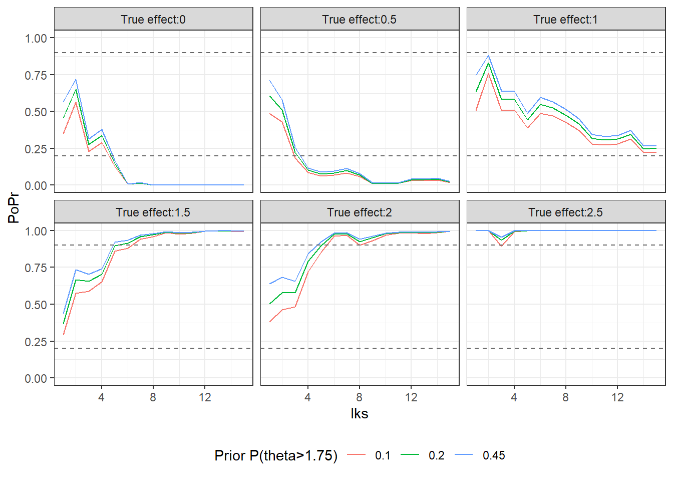
OPT study
Maternal periodontal disease has been associated with an increased risk of preterm birth and low birth weight. The OPT study is a randomized controlled trial aiming at assessing if treating the paradontitis during the pregnance can decrease the risk for preterm birth and low birth weight. Women with paradontitis was randomized to receive treatment either during (treatment) or after pregnancy (control). Sample size is 413 and 410 patients in the treatment and control group, respectively.
The primary aim here is to re-analyse the data by the approach presented in the previous section with the outcome birth weight (g). The data will be analysed on the log scale and presented as geometric mean ratio, such that treatment effect can be interpreted on the percentage scale that is \(\theta=\tau_{2}/\tau_{1}\). Number of looks will be 20 looks that is an interim analysis scheme that consists of 20 looks with the approximate accumulated number of subjects: (21, 42, 63, …, 410 subjects per group, i.e. a total of 42, 82, 124, …, 820). (we remove the last three subjects (subj 821, 822 and 823) for simplicity).
Prior distribution
Use a relatively flat prior with \({\sf P}(\theta>1.20)=0.45\), that is the probability that the effect is at least 20% increase in birth weight is 0.45. This would suggest an unrealistically large treatment effect prior but is used to get the prior really flat.
This prior is achived with \(\sigma_{log\theta}\) = 1.5.
Go/No Go criteria
At each interim look, declare early stopping due to efficacy if: \[\begin{align*} {\sf P}(\theta>1.10|data)>0.9 \end{align*}\] Declare early stopping due to futility/harm if \[\begin{align*} {\sf P}(\theta>1.10|data)<0.2 \end{align*}\] Continue otherwise that is \[\begin{align*} \ 0.2<{\sf P}(\theta>1.10|data)<0.9 \end{align*}\]
Data analysis
Data is available here. I was not able to find inclusion date, so I assume patients were recruited in the order they appear in the data set.
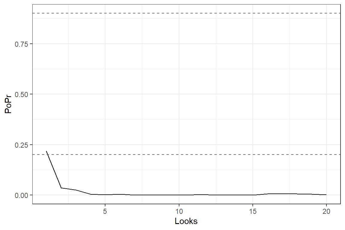
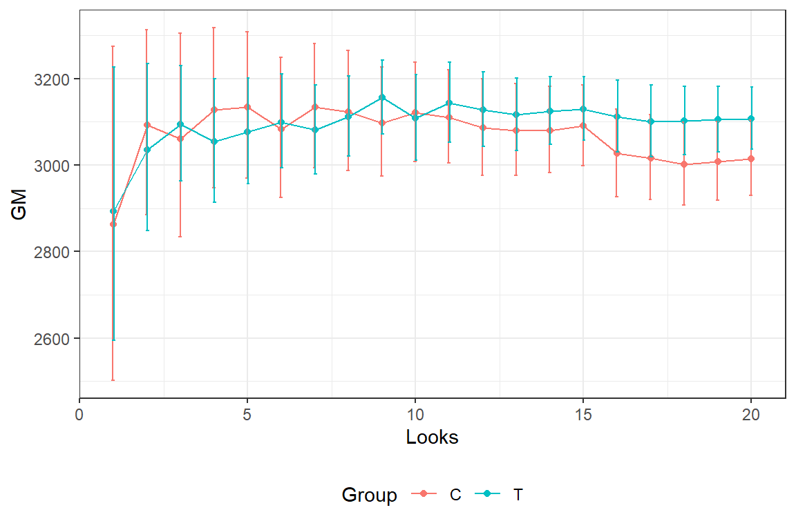
In the graph we see the estimated average (geometric mean) birth weight and 2*SE bars for the different interim looks.
Calculation of posterior probability
The posterior probability of efficacy (as defined here) is extremely small and with the current efficacy criteria the study should be stopped early due to futility (lack of efficacy)