Introduction
This is the third of three posts that address:
1. Predicting the probability of a “positive” (reject \(H_{0}\)) study before running the study
2. Interim analyses during the study
3. Evaluating study data in a meaningful way after the study is completed.
The first post is available here and the second is available here.
Consider the same general linear model as in the previous two posts:
\[\begin{align*} Y_{i}\sim{\sf N}(\tau_{i}, \sigma_{Y}) \end{align*}\] where \(\sum\tau=0\), j=1, 2. The aim is to estimate the treatment effect \(\theta=\tau_{2}-\tau_{1}\). The usual way to report the results from a statistical analysis of data from a finalized clinical study is by the estimated treatment effect, \(\hat{\theta}\), 95% confidence interval, and p-values for testing the null hypothesis \(H_{0}: \theta=0\). From a clinical perspective we are interested in an making statements about the “true” treatment effect \(\theta\) and whether it fulfills requirements for being clinically meaning that is if \(\theta\) is in an interval of values considered to provide a benefit for the patient. Since such statements are made with uncertainty the statements are probabilistic (either in a frequentist or bayesian sense). In this post the interval for \(\theta\) implying a clinical meaningful effect will be taken as given and the aim is to illustrera some approaches to address whether the criteria of efficacy are satisfied.
Frequentist Go/No Go criteria
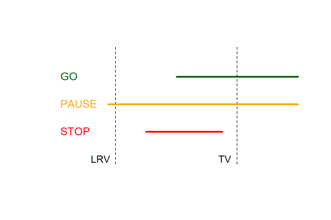
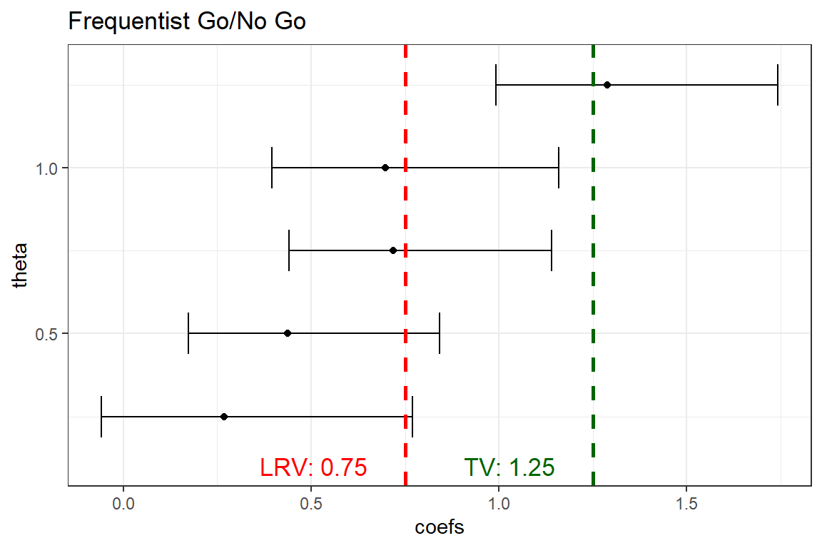
Lalonde et al, 2007 construct a frequentist decision rule do be used to determine whether to continue (GO), pause or stop a drug devlopment program according to the following way. First they define two estimands, \(P^{20}_{\hat{\theta}}\) and \(P^{90}_{\hat{\theta}}\), the 20th and 90th percentiles of the sampling distribution of \(\hat{\theta}\). Second they define the interval of clinically meaningful values of \(\theta\), where the lower and upper part referred to as LRV and TV, respectively.
GO if \(P^{20}_{\hat{\theta}}\)>LRV and \(P^{90}_{\hat{\theta}}\)>TV
PAUSE if \(P^{20}_{\hat{\theta}}\le\)LRV and \(P^{90}_{\hat{\theta}}\)>TV
STOP if \(P^{90}_{\hat{\theta}}\le\)TV
The three scenarios are illustrated in the figure.
Let´s simulate 1000 trial results based on 63 subjects/group, respectively, where \(\sigma\)=2 and \(\theta=\) 0.25, 0.50, 0.75, 1.0 and 1.25, respectively. Set LRV=0.75 and TV=1.25.
library(tidyverse)
# Specifications for the simulations
REP<-1000;
sigma<-2
n1<-63
LRV<-0.75
TV<-1.25
theta. <- c(0.25, 0.5, 0.75, 1, 1.25)

set.seed(123)
# Simulate data
DAT <- tibble(i = seq(1:(REP*(length(theta.))*(2*n1)))  ,
          rep = sort(rep(seq(1:REP), times = (length(theta.))*(2*n1))),
          theta=rep(theta., times = REP*(2*n1)),
          gr=rep(c(rep(0, times=n1), rep(1, times=n1)), times = REP*(length(theta.))),
          Group = factor(gr, labels = c("B", "A")),
          N=rep(seq(1:n1), times=2*REP*(length(theta.))),
          Y = gr*theta + rnorm((REP*(length(theta.))*(2*n1)), 0, 2))
For each true effect and replicate, estimate the percentiles based on assumption of a t-distribution (traditional two-sample confidence interval)
OUT_1 <-   DAT %>%
     group_split(theta, rep ) %>%
     map(~ lm(Y ~ Group, data = .x)) %>%
    # The percentiles from the sampling distribution
  map_df(~ {tibble(LOW = confint(., level = .60)[[2,1]],
                   UP = confint(., level = .80)[[2,2]],
                   coefs = coef(.)[2])})
      OUT_1 <- OUT_1 %>%
        mutate(theta=sort(rep(theta., times = REP)),
              rep = rep(seq(1:REP), times = length(theta.)),
              DECISION = factor(case_when(LOW > LRV & UP > TV ~ 2,
                           LOW <= LRV & UP > TV ~ 1,
                           UP <= TV ~ 0), labels = c("Stop", "Pause", "Go")))
Calculate the percentage of times the different decisions are made and display them in a plot.
OUT_2 <- OUT_1 %>%
group_by(theta, DECISION) %>%
tally() %>%
mutate(Percent = round(100*n/REP, 0 ))
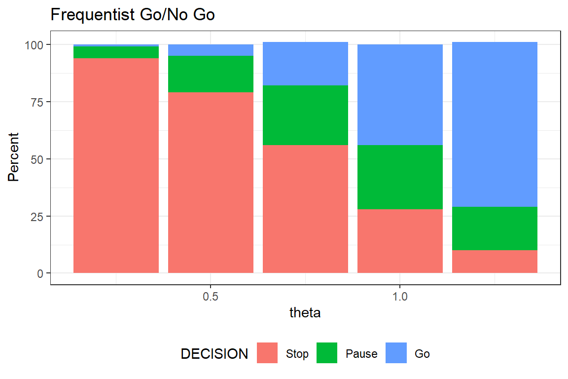
fig1 <- ggplot(OUT_2, aes(x=theta, y=Percent, fill=DECISION)) +
labs(title="Frequentist Go/No Go") +
geom_bar(stat="identity") +
theme_bw() +
theme(legend.position="bottom") +
geom_col(position = position_stack(reverse = TRUE))The larger the true effect, the higher the probability of declaring a Go. When the true effect is equal to TV that is 1.25 the chance of GO is still only 75%. The reason is the relatively small sample size. As mentioned in the previous post, clinical trials often are too small. Hence, sizing a study to achieve 80% power is not necessarily reasonable when the aim is something else - here to have satisfactory expected properties of the Go/No Go criteria.
Bayesian Go/No Go criteria
Use the same framework, but instead of using the percentiles from the sampling distribution calculate instead a posterior distribution and compare these with LRV and TV. Just as in the previous post,
\[\begin{align*} \theta\sim{\sf N}(0, \sigma_{\theta}) \end{align*}\]
For illustration, we use an extremely informative prior, \({\sf P}(\theta> 1.5) = {\sf P}(\theta< -1.5) = 0.05\). The prior implies \(\sigma_{\theta}\) = 0.9 It is not reasonable to use such extreme prior in practice, but we use it here to make differences from the frequentist approach more pronounced (with a highly informative prior, shrinkage will be strong and data will have less influence).
library(Hmisc)

OUT_11 <-   DAT %>%
     group_split(theta, rep ) %>%
     map(~ lm(Y ~ Group, data = .x)) %>%
  map_df(~ {tibble(coefs = coef(.)[2],
                   SE = sqrt(diag(vcov(.)))[2])})
The estimate average treatment effect and it´s standard error are the sufficient statistics (conditional on model and sample size). Use these to derive the posterior average and variance. Since this is a so called conjugate analysis the posterior will be a normal distribution.
OUT_11 <- OUT_11 %>%
            # Posterior mean and SD for theta
  mutate( theta=sort(rep(theta., times = REP)),
          rep = rep(seq(1:REP), times = length(theta.)),
           p_m = as.numeric(gbayes(mean.prior = 0,
                   stat = coefs, var.stat = SE^2,
                   cut.prior=1.75, cut.prob.prior=0.05)[[3]]),
            p_s = sqrt(as.numeric(gbayes(mean.prior = 0,
                   stat = coefs, var.stat = SE^2,
                   cut.prior=1.75, cut.prob.prior=0.05)[[4]])),
  # The percentiles from the posterior distribution
           LOW = qnorm(p=0.2, mean=p_m, sd=p_s),
           UP = qnorm(p=0.9, mean=p_m, sd=p_s),
           DECISION = factor(case_when(LOW > LRV & UP > TV ~ 2,
                           LOW <= LRV & UP > TV ~ 1,
                           UP <= TV ~ 0), labels = c("Stop", "Pause", "Go")),
          theta=sort(rep(theta., times = REP)),
              rep = rep(seq(1:REP), times = length(theta.)) )
Calculate the percentage of times the different decisions are made and display them in a plot.
OUT_21 <- OUT_11 %>%
group_by(theta, DECISION) %>%
tally() %>%
mutate(Percent = round(100*n/REP, 0 ))
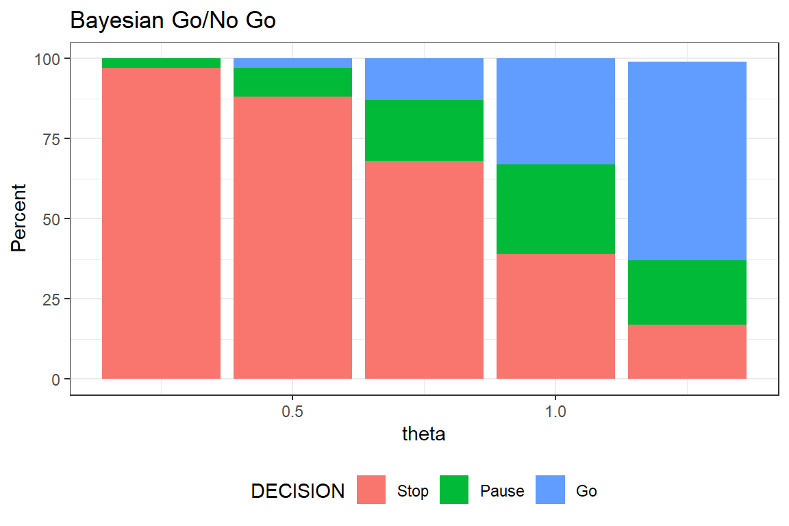
fig2 <- ggplot(OUT_21, aes(x=theta, y=Percent, fill=DECISION)) +
labs(title="Bayesian Go/No Go") +
geom_bar(stat="identity") +
theme_bw() +
theme(legend.position="bottom") +
geom_col(position = position_stack(reverse = TRUE))The despite we used a highly informative prior, the posterior will be more or less solely driven by data. If you compare the two figures you´ll see that the probability of GO is lower in the bayesian analysis. For example when \(\theta\)=1 then probability of GO is 44% and 33% for the frequentist and bayesian approach, respectively, which is due to a strong shrinkage effect of the prior.
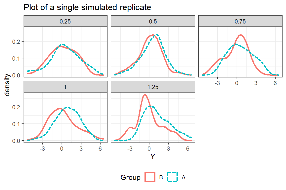
Look at a single study in more detail
Let us use one of the 1000 simulated studies (but we still allow the true effect to be of different size).
We see that the signal-to-noise ratio is lower than one might intuitively would expect from a large value of \(\theta\).
Frequentist analysis
All scenarios result in a STOP except for \(\theta\)=1.25 that results in a GO.
Bayesian analysis
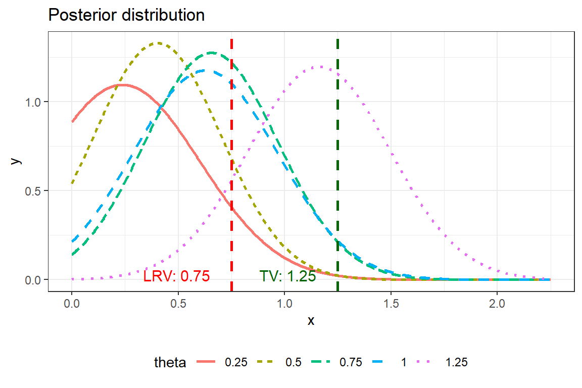
When we have a single study it is convenient to use the whole posterior distribution to support decision making. Frank Harrell suggest a great of visualisation here.
This plot can can give you information on for example P(\(\theta\)>TV|data) that is information that is highly relevant for decision making. This is the area to the right of the TV-line in the figure below. We see that for TV=1.25, P(\(\theta\)>TV|data) is relatively small for all true values of \(\theta\). This is again due to the aggressive shrinkage of out prior.
| 0.25 | 0.5 | 0.75 | 1 | 1.25 |
|---|---|---|---|---|
| 0.0027 | 0.0024 | 0.029 | 0.033 | 0.4 |
Concluding remarks
When I several years ago was introduced to the Lalonde´s concept I was told it was in some sense semi-bayesian. I actually have difficulties to understand the semi-bayesian in the approach since the statistical model is purely frequentist. But the approach is excellent to combine with Bayesian thinking. This has also been done by the book by Dmitrienko et al. If you have little or skewed data, \(P^{20}_{\hat{\theta}}\) and \(P^{90}_{\hat{\theta}}\), can be estimated by bootstrapping technique. But I think it would be even better to use a bayesian approach a combine it with a semi-parametric model such as ordinal regression, as it demonstrated here. I have here taken LRV and TV as given and haven´t discussed how how to determine them.